Probabilistic Clustering - Mixture Model
Introduction
Think Generatively
The idea is simple, assuming there are 3 clusters, defined by 3 multivariate Gaussians (it can be other distributions) with observed data points, as with the example plotted below (which we will use throughout this)
We want a model that can generate data that looks like the 3 clusters
Now say we know the 3 Gaussians, we then can generate the data by:
- Select one of the Gaussians
- Sample data from this Gaussian
But how do we define the 3 Gaussians that is supposed to be unknown? We can do this by deriving the model likelihood function and find the parameters that maximise it! Just like the classic MLE!
This is called a mixture model because we assume that the data is sampled from a mixture of several individual density functions
# Generate simulated data to test model----
set.seed(234)
# cluster 1, 100 samples:
clus_1 = rmvnorm(100, mean = c(0,5), sigma = matrix(c(0.5,0.1,0.1,5),ncol=2))
# cluster 2, 200 samples:
clus_2 = rmvnorm(200, mean = c(-7,5), sigma = matrix(c(4,0.1,0.1,0.5), ncol = 2))
# cluster 3, 50 samples:
clus_3 = rmvnorm(50, mean = c(-4,-0), sigma = matrix(c(1,0.7,0.7,1), ncol = 2))

# put them together for plotting

# for column on actual cluster
actual = c(rep(1, nrow(clus_1)),rep(2, nrow(clus_2)),rep(3, nrow(clus_3)))

train_df = as.data.frame(rbind(clus_1,clus_2,clus_3))

train_df$actual_clus <- as.factor(actual)

colnames(train_df) <- c("X1","X2","actual_clus")

# plot the distribution:

# create function that generate data for contours
set.seed(23)

create_data_for_mvnorm_contour <- function(n, mean, sigma) {
  d <- as.data.table(rmvnorm(n, mean = mean, sigma = sigma))
  setnames(d, names(d), c("x", "y"))
  testd <- as.data.table(expand.grid(
    x = seq(from = min(d$x), to = max(d$x), length.out=50),
    y = seq(from = min(d$y), to = max(d$y), length.out = 50)))
  testd[,Density := dmvnorm(cbind(x,y), mean = colMeans(d), sigma = cov(d))]
  return(testd)
}

# create data to plot contours
clus_1_contour_actual <- create_data_for_mvnorm_contour(1000, mean = c(0,5), sigma = matrix(c(0.5,0.1,0.1,5),ncol=2))
clus_1_contour_actual$actual_clus = 1
clus_2_contour_actual <- create_data_for_mvnorm_contour(1000, mean = c(-7,5), sigma = matrix(c(4,0.1,0.1,0.5), ncol = 2))
clus_2_contour_actual$actual_clus = 2
clus_3_contour_actual <- create_data_for_mvnorm_contour(1000, mean = c(-4,-0), sigma = matrix(c(1,0.7,0.7,1), ncol = 2))
clus_3_contour_actual$actual_clus = 3

contour_actual <- rbind(clus_1_contour_actual,clus_2_contour_actual,clus_3_contour_actual)
contour_actual$actual_clus <- as.factor(contour_actual$actual_clus)


ggplot(train_df, aes(x=X1, y=X2, group=actual_clus, col=actual_clus))+
  geom_point()+
  geom_contour(data = contour_actual, aes(x,y,z=Density), size = 1, linetype = 2, alpha = 0.3)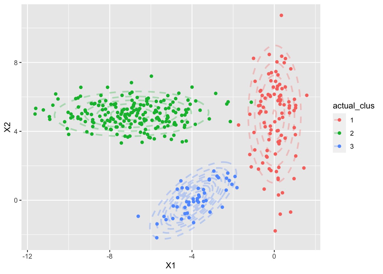
Figure 1: Our simulated datasets - with three 2-D Gaussians
What is wrong with K-means?
K-means is one of the most popular clustering methods out there, it clusters observations by minimizing (up to local minima) the within-group dissimilarity.
However, it has its disadvantage compared to using mixtures
K-means cluster definition is crude as it uses one point (the centroid) to represent the whole cluster. Using mixtures incorporate a notion of shape
Since each cluster is represented as a probability density using mixture models, it can have various shapes and data form (e.g. binary dataset with Bernoulli distributions)
A posterior probability is the output of the model, hence we know the probability of an observation belongs to each cluster given parameters. This gives us a confidence indication on our clustering and also imply that using mixtures, clusters are less sensitive to outliers
Because there is a dataset likelihood function, we can optimise K too. In K-means, this is impossible
K-means fails in our simulated dataset
We can see some misclassification mainly for cluster 2 as cluster 1 if we use K-means
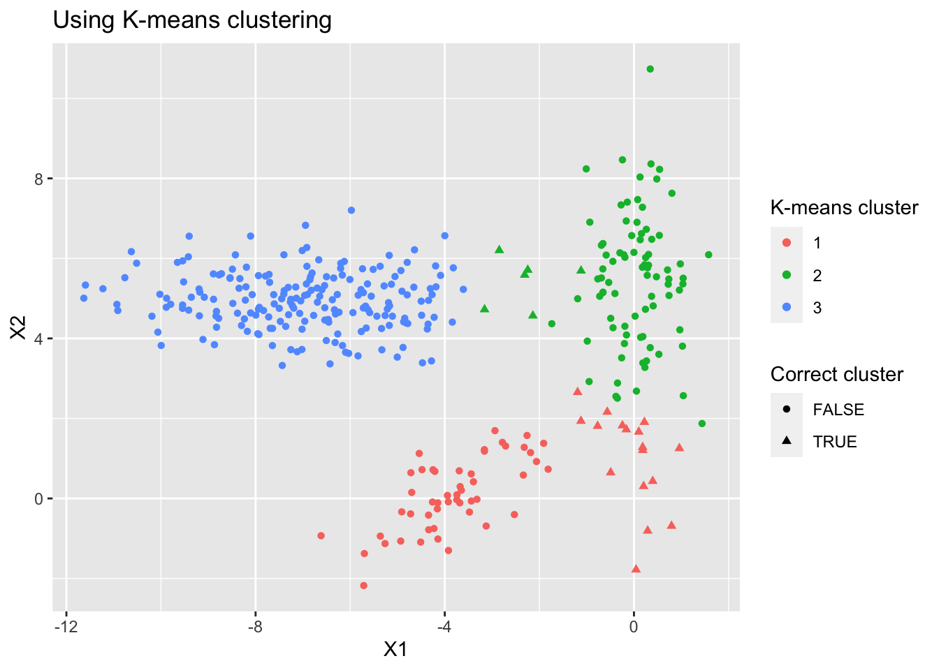
Figure 2: K-means fails to capture the shape of clusters
Finding Parameters
The way to find and optimise parameters is somewhat technical, I encourage you to read the references at the end of this markdown, and you are more than welcome to look into my Probabilistic Clustering.Rmd in repo
In summary, we need to do the following:
- Define our dataset likelihood
- Unfortunately, we will end up with log-sum expression which is hard to optimise, so we use Jensen’s Inequality and maximise the lower bound instead
- We take partial derivatives with respect to each parameter and equating to 0 and end up with two sets of expressions which require to solve with an iteration method called - Expectiation Maximisation (EM) Algorithm
The Result
Summary of the model iterations
The plot below shows the initialised 3 Gaussians in green, and the resulted Gaussians that the model converges to using EM Algorithm in blue, compared with the actual Gaussians in red.
Resulting Gaussians are very close to actual!!
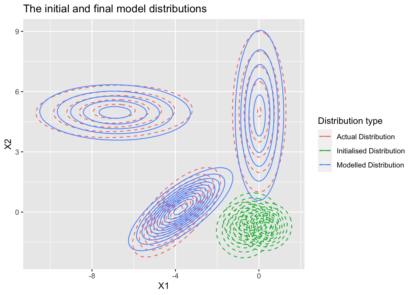
Figure 3: Change in the Gaussians model likelihood
The model output with posterior probabilities for each cluster (head)
| Simulated observation | X1 | X2 | Actual Cluster | Posterior Probability for Cluster 3 | Posterior Probability for Cluster 2 | Posterior Probability for Cluster 1 | Max. Posterior | Predicted Cluster | Same as Actual |
|---|---|---|---|---|---|---|---|---|---|
| 1 | 0.3969151 | 0.4323799 | 1 | 0.0000138 | 0.0000000 | 0.9999862 | 0.9999862 | 1 | 1 |
| 2 | -1.0088671 | 8.2384402 | 1 | 0.0000000 | 0.0000044 | 0.9999956 | 0.9999956 | 1 | 1 |
| 3 | 1.0353373 | 5.3629194 | 1 | 0.0000005 | 0.0016125 | 0.9983870 | 0.9983870 | 1 | 1 |
| 4 | 0.0445500 | -1.7810088 | 1 | 0.0000000 | 0.0000000 | 1.0000000 | 1.0000000 | 1 | 1 |
| 5 | -0.3808923 | 2.5511852 | 1 | 0.0160735 | 0.0000866 | 0.9838400 | 0.9838400 | 1 | 1 |
| 6 | 0.0783891 | 7.4702457 | 1 | 0.0000000 | 0.0000080 | 0.9999920 | 0.9999920 | 1 | 1 |
And the model result plot
We can see the model only put two observations in the wrong group, much better than K-means
The plot also annotates the observations with the lowest class posterior probability
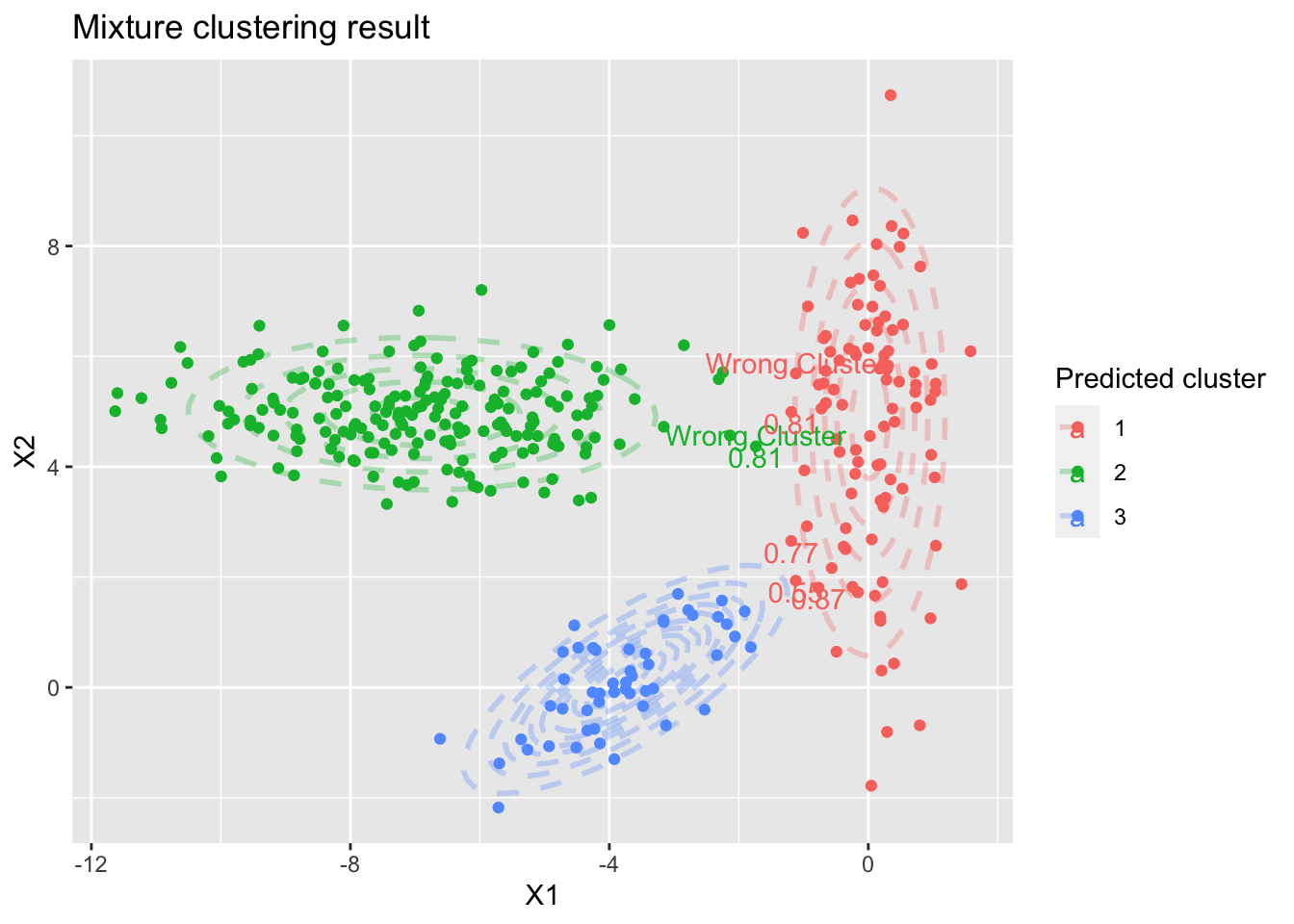
Figure 4: The resulting clusters
Finding K: the number of clusters:
- Intuitively we can use K that maximises the dataset likelihood. However, as K increases, likelihood increases monotonically.
- This is because, with more distributions, data will lie near the mode of the pdf, hence likelihood with increase. Similar to overfitting
- We can use cross-validation to find the best K
Running the model for different values of K with 10-folds CV (again feel free to read the code in Probabilistic Clustering.Rmd in repo), we find that mean test log-likelihood is largest when K = 3 (although K = 4 is nearly as good), which is the correct number of clusters
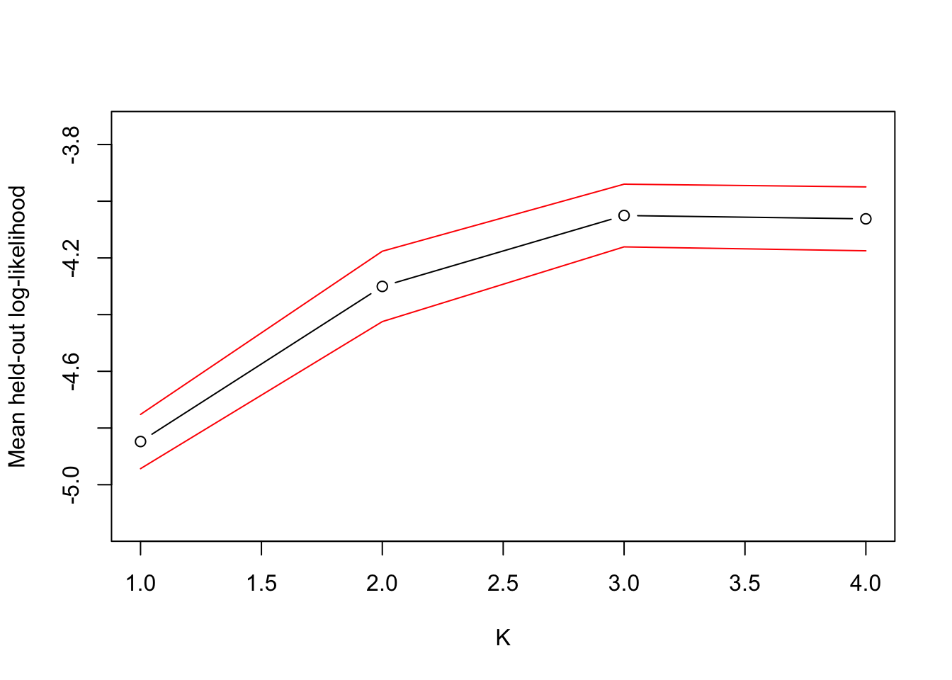
Figure 5: Mean held-out log-likelihood for different values of K
Limitations
There are several limitations
- No extensive packages for this algorithm: mclust in R is the closest but with limited flexibility (only support normal mixture model and BIC for selecting K)
- Like k-means, the algorithm only finds local optima, testing multiple starting points needed
- Some data forms might be better with kernelized k-means, e.g. radials
Extentions
There are serveral usage extensions
- Other forms of mixture components: e.g. Bernoulli for binary data
- Regularise param estimates by setting likelihood x prior
Key References
Simon Rogers and Mark Girolami. A First Course in Machine Learning. CRC Press, second edition, 2017.
Gareth James, Daniela Witten, Trevor Hastie, Robert Tibshirani. An Introduction to Statistical Learning : with Applications in R. New York: Springer, 2013.